

If you’re like me, you’re always looking for a way to save money in your AWS environment. However, this is not always as easy as it sounds. We’re often asked to develop solutions for complex projects which present the types of challenges and opportunities we love to solve...but we're also asked to keep an eye on the budget.
For workloads deployed to AWS, one of the largest costs in most organizations is their EC2 instance costs, usually exceeding 60-75% of the total AWS bill. So, with that in mind, how can we utilize the different EC2 instance purchase types to get the most bang for our buck with a compute intensive workload like image optimization? For example, can we run reliable image optimization workloads on EC2 spot instances.
Spot instances have the possibility for huge savings, usually between 60-90% savings over On-Demand pricing. But how can we use spot fleets for the highly available and dynamic workload of CDN Image Optimization at the scale of 1,000 images per second? Let’s find out.
Spot Instances
We know EC2 spot fleets have the potential for the greatest savings, but they are also the most volatile, requiring the workloads they serve to be able to handle interruptions gracefully. The main use case for spot fleets is to handle burst requests from a task source like a message queue, such as AWS SQS. In this type of architecture, a certain proportion of the compute power comes from reserved EC2 instances. When additional computer power is needed, your environment provisions a spot fleet instance. If the spot backed instance is terminated mid task, the message returns to the queue to be process by the next available worker. But what if we flipped this on its head?
One way to handle the inherent volatility of spot is to widen the number of spot pools and monitor the workload’s performance. If performance degrades, we can trigger a scaling action to spin up On-Demand instances; essentially the reverse of the example above. In our case of the CDN Image Optimization system, a spot fleet of 4 instance types spread across 3 availability zones yields a high probability of having a fulfilled spot request. Further, backing the spot fleet with an auto scaled on-demand system fills any gaps where spot fleet cannot keep up with the load or where spot fleet is not available.
Let’s take a quick look at this architecture.
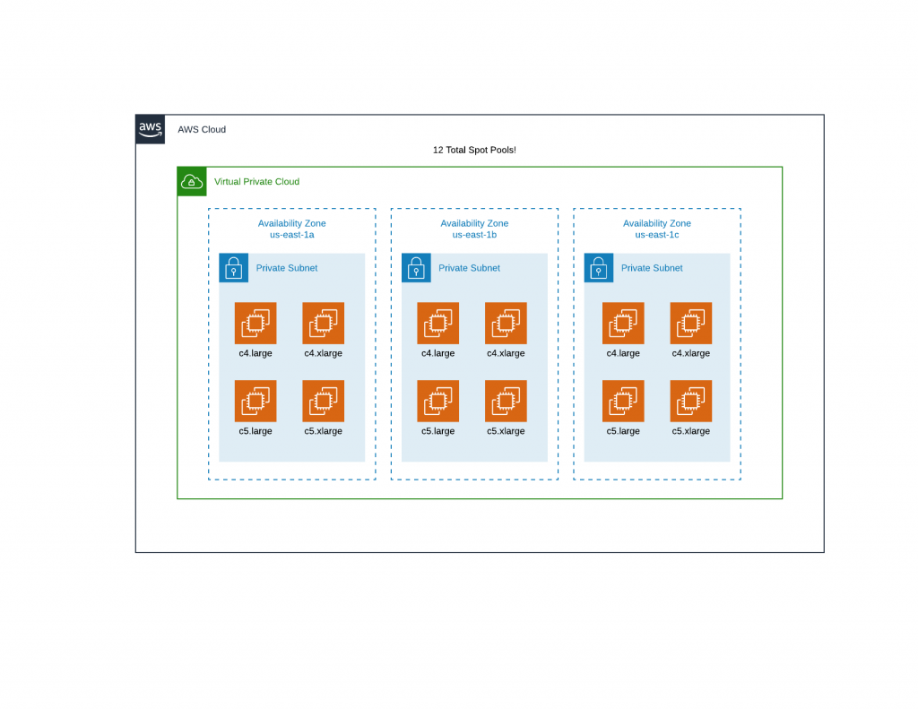
Spot Fleet “pools” are made up of an EC2 instance type in the desired availability zone. In the case of the Image Optimization, we will be using 4 Instance types (c4.large, c4.xlarge, c5.large, c5.xlarge) across 3 availability zones (us-east-1a, us-east-1b, us-east-1c), leaving us with 12 spot pools.
 Choosing the right instance type for your spot fleet will also dramatically change your cost savings. For image optimization, our workload will be CPU intensive, so we are choosing AWS’ compute optimized “C” class. This infrastructure will serve containers which will have resource constraints enabled. This will set the limit on the maximum amount of CPU and memory a container can use to 1 vCPU and ~2GB of memory, allowing us to fit either 2 containers (on the “large” instance types) or 4 containers (on the “xlarge” instance type) on each instance. Containerized applications don’t care where they live, as long as there is room for them to “land”. We could choose even cheaper instance types with similar specs, namely the T instance type (T3.Medium) where the cost savings are greatest. T class instances on paper have similar specs, but in reality have greatly diminished CPU power.
To read more about the T class burstable CPU, check out this page.
Containerize for Spots
Containerized applications go very well with spot fleets. They are both ephemeral (no persistent data), both are cheap, and both can grow quickly and easily as your load increases. For our Image Optimization use case, it would be handling 1,000 requests per second. At that rate, static infrastructure would be too costly, serverless infrastructure is not as performant, and serverless integrations with AWS CDN CloudFront, through the use of AWS API Gateway, becomes cost prohibitive.
For our deployment, we settled on 2 main containers.
The first one acts as a reverse proxy, we are calling it “LogicProxy”. Here we apply all the needed logic to each request such as source image location, user account subscription status, user account limits, and more. This container was created using Go Language for its speed, efficiency, and small footprint. If you would like to learn more about creating Go reverse proxies, check out the great video from Julien Salleyron: How to write a reverse-proxy with Go in 25 minutes.
The second type of container is the image optimizer. For this we will use ImgProxy created by DarthSim and evilmartians.com. This software was chosen for its speed, security, reliability and its great support and community. DarthSim and the other Developers have created an amazing containerized solution for image optimization that, when scale horizontally, will serve our use case in a very cost-effective manner. The best part is, this system is already containerized and highly customizable through environment variables, which means no need to maintain a separate copy of the code, unless you want to. Here are links to the code on GitHub and Evil Martians.
For our purposes, ImgProxy will remain a blackbox, meaning we will not be forking the code, but instead we will be referencing the “latest” public docker container build.
Backing Spot with On-Demand
Backing spot fleets with on-demand may seem counter intuitive, but it can result in a robust and reliable workload platform. Why not back with reserved instances? Again, the idea is to keep this system as cheap as possible and thus the on-demand should only be used when the spot fleet cannot keep up with the load, or spot cannot be fulfilled.
When scaling spot fleet workloads, it is important to find the key metric(s) that your spot fleet should use to trigger auto scaling actions. Once this metric(s) is chosen, we can adjust the threshold and responsiveness for our on-demand scaling actions so they are only used when the spot request cannot keep up (or cannot be fulfilled). We will learn more about using these later in this blog.
Overall Architecture
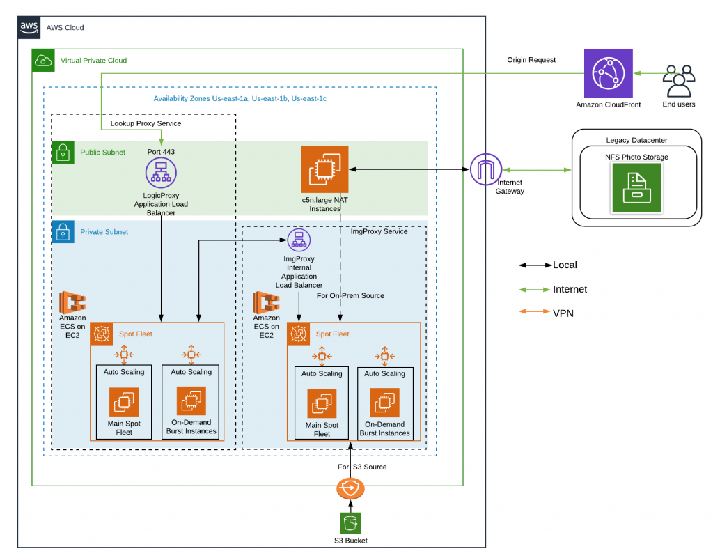
Now let’s look at how each of these pieces will fit together to complete our AWS Image Optimization workload architecture.
This image optimization system will be paired with AWS CloudFront. CloudFront will be used to optimize the experience of the end use, but if there is a “cache miss” meaning CloudFront doesn’t have a copy of the requested file in its system, it will need to go to the origin to get it.
Next, origin requests are made to our public LogicProxy load balancer which distributes the load to the various containers. LogicProxy does its work, applying filters, checking user status, etc. to decide what the optimized image should look like. It passes those settings to the ImgProxy which formats the image and sends it back to LogicProxy which sends the resulting file (filters and attributes applied) to CloudFront to be served and cached.
 When looking at the diagram above, you will notice something interesting.
Why did we choose ECS over EKS? The short answer is price. ECS has no additional cost for the service. You are only charged for the worker instances you connect to the cluster. Whereas EKS has a price of ~$146/month. Additionally, ECS has simpler and easier integration with other AWS services such as CloudWatch, Auto Scaling, and Application Load Balancers. Each of the EC2 groups depicted, though separate groups in the diagram, are actually a single group of Spot fleet workers and a single group of On-Demand Burst workers, both of which are a part of a single ECS Cluster.
Next, you will notice EC2 based NAT Instances, and as with the ECS/EKS debate, this came down to cost. The original image source can be in one of two places; in an on-premises datacenter, or in AWS S3 bucket. A majority of the content is still located on-premises and is internet accessible, so accessing it is easiest over the internet.
As with any private network resource, accessing the internet requires a NAT Gateway. But AWS’ NAT Gateway service costs half as much as the infrastructure serving the requests, so something had to change. With the use of NAT Instances, we were able to cut the NAT cost nearly in half and since it should be temporary, we felt it would be a good fit. NAT instance workloads are network intensive, and again cheap T class instances are not a good fit because of their limited network throughput. We needed a compute and network optimized instance type and the best fit (and best price) is the C5n.large.
CloudWatch Dashboarding and Alarms
We decided to use CloudWatch for our metric analysis for its ease of integration with AWS ECS. We created dashboards and alarms for our pertinent metrics and set the scaling thresholds based on the business requirements. In our use case, we wanted to see the average response time between 0.40-0.65 seconds for image optimization requests, along with other metrics that help show the overall health of the environment.
Let’s look at the some of the key metrics we chose to display and why.
Average response time is our key business and scaling metric so that’s where we look first to see if the workload is healthy. Since our autoscaling actions are based on this metric, we expect some volatility in this graph.
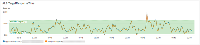
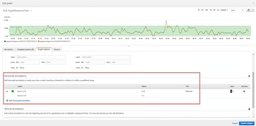
The filled green section is our target, and ideally the volatility we stay within the bounds of the target. This view can be easily created in CloudWatch with the use of “Horizontal Annotations”. To edit your graph, go to “Graph options”, add your values, and select the fill as “Between”.
We can use this same metric and create alarms for the different scaling actions (spot fleet and on-demand). We created 4 alarms, 2 for scale out (1 for spot and 1 for on-demand), and 2 for scale in (1 for spot and 1 for on-demand), with the main difference being the threshold.
The spot fleet has a more responsive alarm (1 out of 1 failures) with a threshold of 0.65 seconds while the On-Demand has a less responsive alarm (3 out of 3 failures) with a threshold of 1.5 seconds. This allows for some fluctuations in response time while we wait for spot fleet resources to come online. If the spot fleet cannot keep up with the requests, On-Demand will trigger and scale out, adding more workers to our ECS cluster allowing more containers to be deployed.
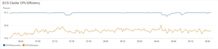
Since we are using AWS ECS, we also have the ability to check our CPU efficiency. The blue line below indicates how well we are using the the underlying EC2 infrastructure. We always want the blue line to be at or very near 100%. Here we also added the ECS cluster CPU utilization for further insights on the cluster’s utilization.
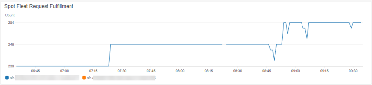
Spot Fleet Fulfillment is an important indicator of how our spot fleet is scaling with our load. We expect these vertical “jumps” to correspond to the stepped based scaling policy which is detailed later.
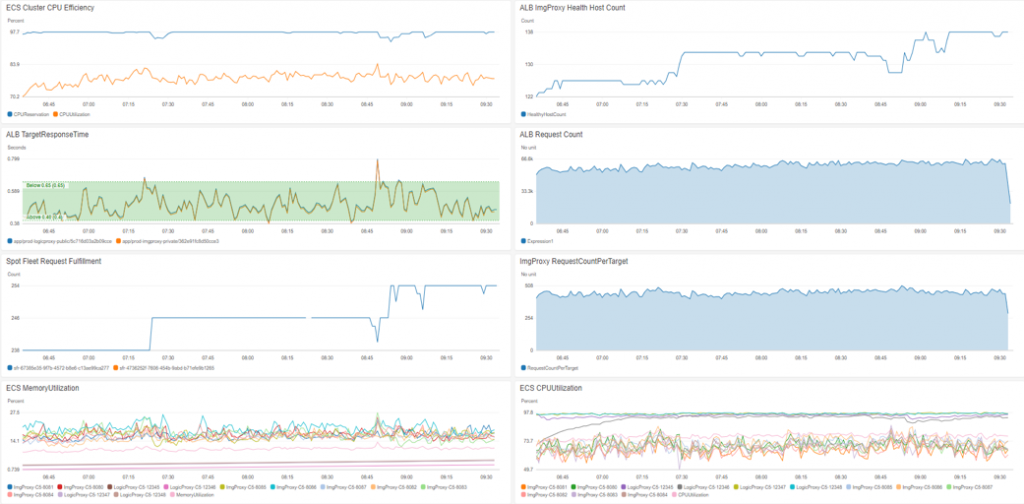
Combining all of our graphs into a single view provides a snapshot of the overall health and performance of the environment.
Spot Instance Request Details
Config Types
Spot fleet configurations have 2 types; CPU requests and Instance requests. Because we are containerized, and computer intensive, we went with CPU based spot request provisioning to have more flexibility on the type of instances used in our spot fleet. With CPU based requests, we don’t care about the type of instance, or even the size (large vs xlarge), we care about a distributed and cost-efficient spot fleet.
Savings
With the spot fleet request dashboard in the AWS Console, we have visibility into the savings achieved. Here is a screenshot of the average hourly savings for sub 500ms response times of 1,000 image optimization requests per second, just over $4.50/hour.

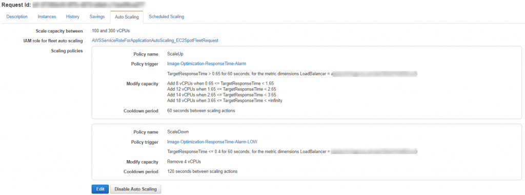
Autoscaling
Spot fleet also has 2 types of scaling policies; Target Tracking and Step/Simple Scaling. Target Tracking scaling policies allow you pick a metric (such as average spot fleet CPU utilization) at which the spot fleet will scale up and down to try to maintain a set value. This sounds like it would be exactly what we want! But sadly, the metrics we can choose from are limited.
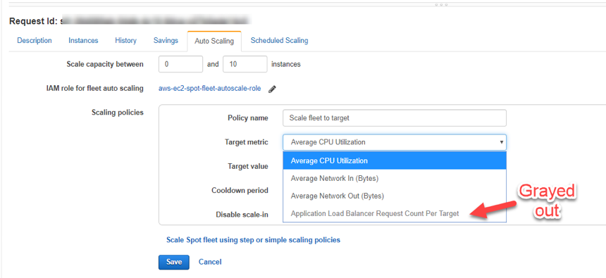
Also note that if you do not associate the Spot Fleet to a load balancer on creation, you will not have access to the Load balancer request “Count per Target” option in this type of scaling request.
In our image optimization workload, we are using a custom metric for our business and scaling trigger so we’ll have to use the Step or Simple Scaling type policy. We chose to add “Steps” to the scaling action because it gave us the ability to ramp up our spot fleet quicker as the response time surpassed the threshold at greater intervals.
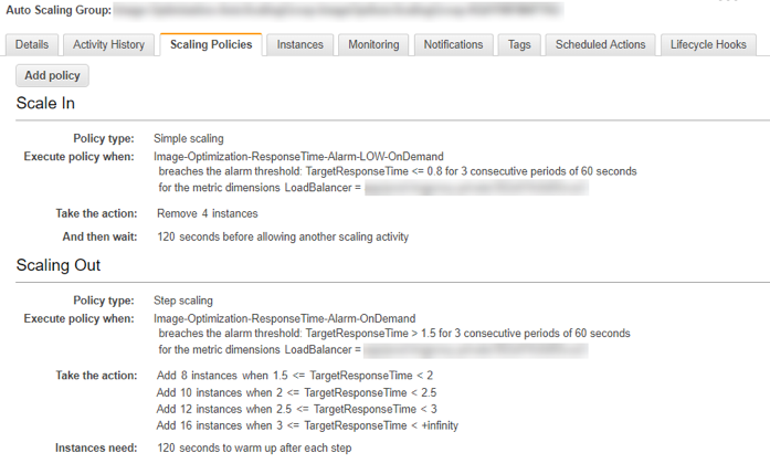
On-Demand Scaling
Our on-demand scaling policy is organized in a similar manner to the spot fleet scaling policy. Keep in mind that these are scaling instances (c4.large) not CPUs and that this scaling action is for emergency purposes only. We want to ramp up quickly if spot cannot keep up, thus taking more aggressive steps.
Final Thoughts
With this implementation, we have a working, highly reliable, containerized workload at scale, done with AWS’ cheapest class EC2 instances. But what are some lessons learned?
Spot fleet configurations do have some limitations. Referencing launch configurations in the process limits the customization (such as tags) that can be applied to the instances at their creation (for example having a naming standard for your spot fleet).
When in production, you may want to do more subtle rolling changes of the spot fleet. I recommend doing a rolling update where you create a new spot fleet (CloudFormation is possible), then slowly ramp down your old spot fleet until it can be deleted.
Next, if you decide to tie your spot to a load balancer (for load balancer metric-based scaling), the instances will be attached to the load balancers target group automatically and use port 80 as default. If your application is not running on 80, your unhealthy target count will be unusually high.
With that said, this deployment has proven to be a robust, cost-efficient, and reliable architecture that can be replicated for many other workloads in AWS.